
◷ Reading Time: 10 minutes
We were inspired by the Analyzing Employees DMC Challenge to create models designed to analyze an organization’s workforce. This challenge aims to “help an HR office create a rules-based service to analyze its employees” by setting up a decision management service that answers a series of questions based on the given employee data.
Scenario
Imagine you’re an HR professional tasked with analyzing employee data to gain valuable insights. Currently, this process might involve manually sifting through spreadsheets or writing custom code. But what if there was a more efficient and flexible way to analyze your workforce?
This scenario dives into how FlexRule Designer can be used to create a solution for HR analytics. This model will take employee data delivered as a JSON request and answer your burning questions:
- Total Workforce Size: Get a quick snapshot of your total employee count.
- Employee Demographics: Analyze the average number of children employees have, identify the number of single employees, and understand the overall salary distribution (average, minimum, and maximum).
- Location Analysis: Discover the states where employees reside and identify employees living in certain zip codes.
- Top Earners: Pinpoint the top 20% highest-paid employees.
This scenario will showcase how FlexRule Designer tackles these analytical tasks step-by-step, transforming raw employee data into actionable insights that can inform better HR decisions.
This challenge is posted in DM Community and you can find more details in here.
Lets take a look on how we can implement this scenario in FlexRule Designer.
We will explain 4 different ways to approach this scenario.
- Decision Graph Approach
- Decision Graph and Decision Table Approach
- Decision Table Approach
- Interactive Shell Approach
Decision Graph Approach
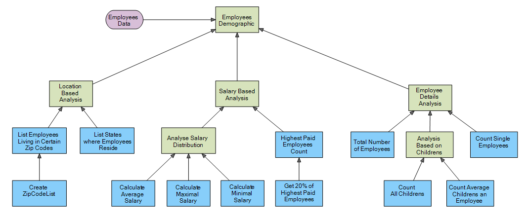
This approach consists of a major decision outcome and its sub-decision nodes and shows the decision hierarchy of how a particular decision will be made. This model take the input(Employees Data) as JSON. Each Decision Node marked in light blue consists of an expression that derives the answer to a question. And those answers will be assign to a output parameter called Results.
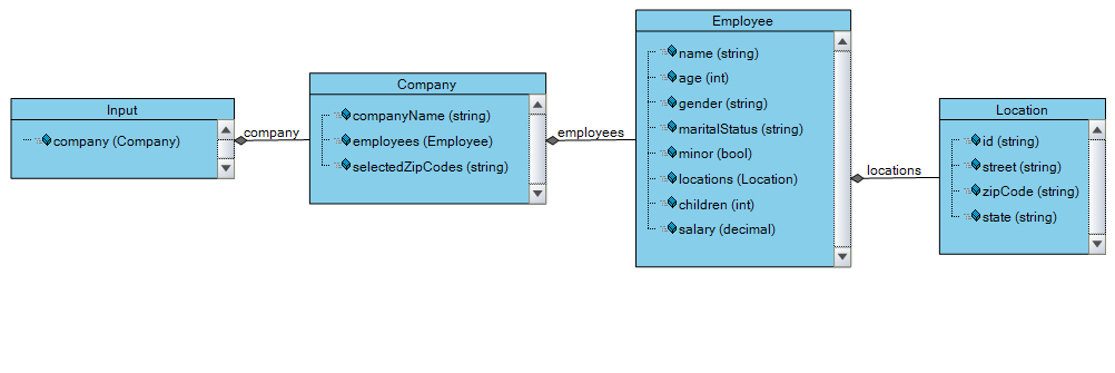
Input and Output Structure
Inpt data structure in the Fact Concept as follows. This Fact Concept can be created by importing the JSON data file.
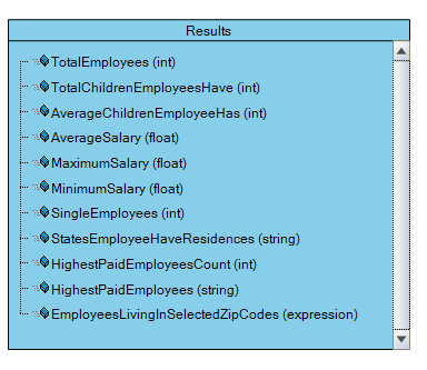
The output data structure(Results) is designed based on the nature of the model output.
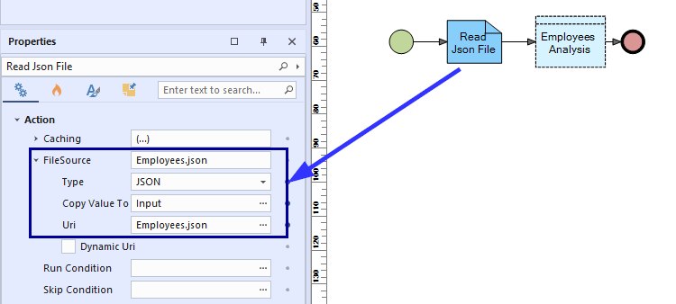
Read the JSON file
In order to read the JSON file, we used File node and set the URI to the JSON file. The JSON data will be saved using a parameter called Input. Then as the next step we can send that parameter as an input for the above mentioned Decision Graph.
Decision Graph and Decision Table Approach
In this approach, a Decision Graph as well as a Decision Table is involved to derive an outcome similar to the previous approach. Let’s have a look at each step in detail.
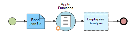
Read the JSON file is exactly similar to what we discuss previously.
Apply Functions
This decision node is designed as a Natural Language document.
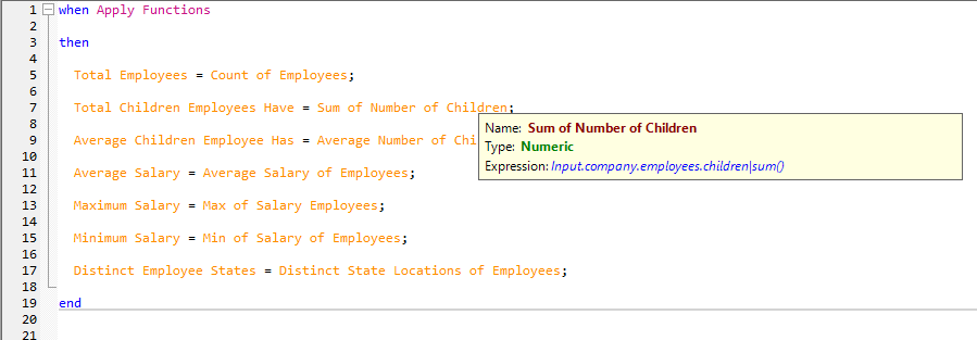
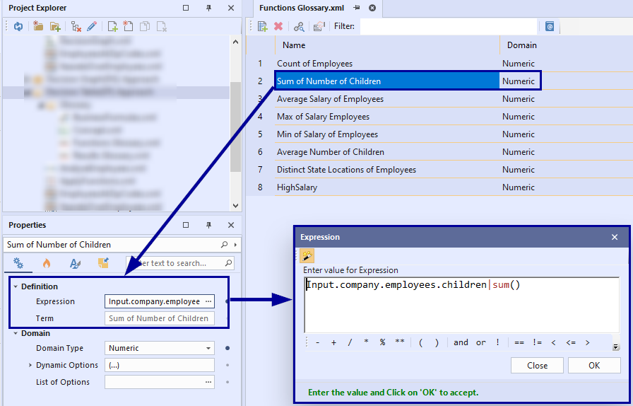
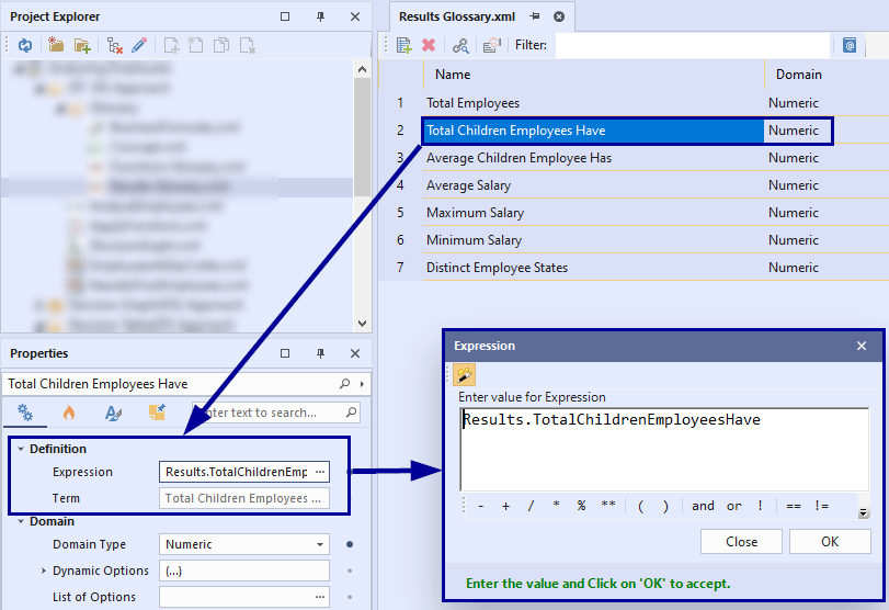
There are 2 Business Glossary documents referenced with this Natural Language document in order to refer those business terminologies with relevant expressions. When you hover to a specific business term, it will show you the linked expression as shown in the image above. The main benefit of using a Business Glossary is the reusability of business definitions.
Employees Analysis
This decision is a combination of 2 sub-decisions which is modeled as a Decision Graph.
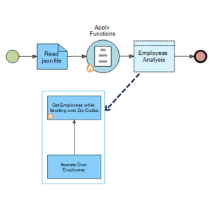
Iterate Through Employees
The first Decision node is responsible for iterating over Employees collection and accessing the employee specific attributes. Lets have a look on this logic implementation.
This logic is modelled as a Decision Table.
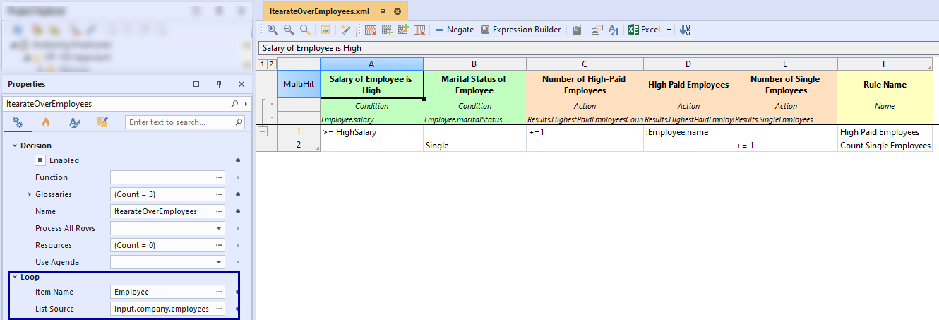
Loop: This loop iterates over each employee within the “Input.company.employees” section of the input JSON data. “Employee” becomes the current employee being examined during each iteration.
Rule: High Paid Employees: This rule checks if the current employee’s salary (“Employee.salary”) is greater than or equal to a threshold value stored in “HighSalary” (defined in a business glossary).
- If true:
- The count of high earners in “Results.HighestPaidEmployeesCount” is incremented by 1.
- The employee’s name is added to the “Results.HighestPaidEmployees” collection.
Rule Count Single Employees: This rule checks if the current employee’s marital status (“Employee.maritalStatus”) is equal to “Single”.
- If true:
- The count of single employees in “Results.SingleEmployees” is incremented by 1.
Create ZipCode List
Before moving to next decision, ZipCode list needs to be created. We used a pre-execution event to create the Zip Code list as follows.
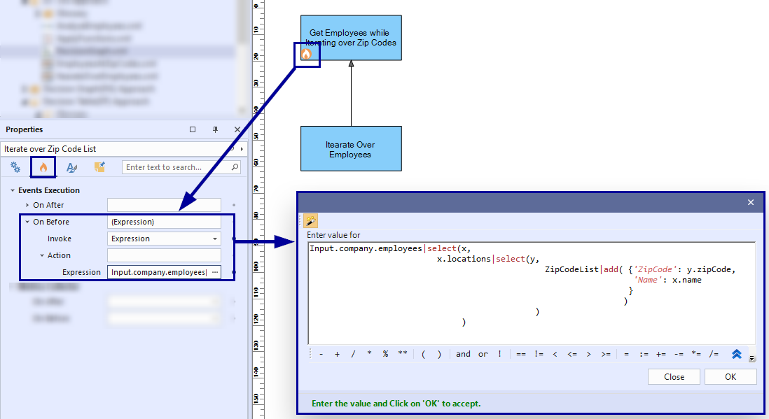
Iterate Through ZipCode List
In this decision node, the Zip Code list will be iterated in a decision table.
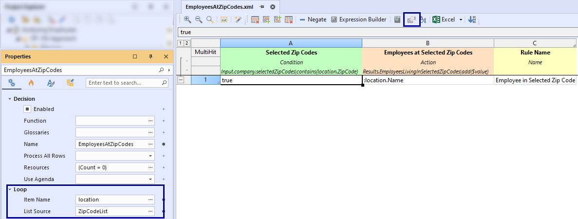
Loop: This loop iterates over a list named “ZipCodeList,” defined previously. During each iteration, “location” holds the current zip code being examined.
Rule: Employee in Selected Zip Code: This rule checks if any employees’ location has a zip code listed in the “selectedZipCodes” attribute in the input.
- The expression uses the “contains” function, implying “Input.company.selectedZipCodes” a collection of zip codes in input JSON, matches the current location’s zipcode:
- Then:The employee’s name is added to the “Results.EmployeesLivingInSelectedZipCodes” collection.
Decision Table Approach
In this approach, we used only Decision Tables are involved to derive an outcome similar to the previous approaches. Let’s have a look at each step in detail.
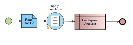
Read the JSON file, and Apply Functions is exactly similar to what we discuss previously. Lets have a look on Employees Analysis decision node.
Employees Analysis in a Decision Table
This Decision Table is mostly similar to what we discussed in the previous approach other than the last rule.
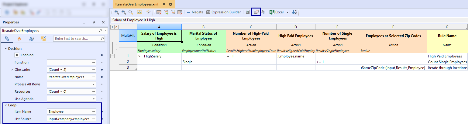
Rule: Iterate through locations: In this rule, a separate embedded model named “SameZipCode” is called using parameters “Input”, “Results”, and “Employee” data for processing.
Embedded Model
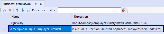
This embedded model is defined in a Business Formula as follows. As an embedded model, the EmployeesAtZipCodes Decision Table is referred to iterate thorugh locations.
Interactive Shell Approach
In this approach we don’t build any models, instead, we analyze the data using the FlexRule Interactive Shell which may be suited for someone with a data science background. Here we’ll use monadic operators similar to using a Python or R shell to manipulate and analyze data.
The first step is to open up the interactive shell: 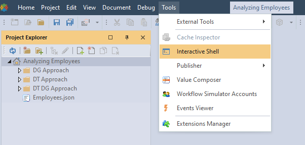
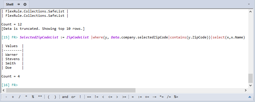
The JSON file can be imported into the shell, and monadic operations can be performed on it. In the following code, we demonstrate selecting employee names associated with selected zip codes designated by the JSON input.
We start by reading the JSON file as a variable called Data.
Data := fileReadText("Analyzing Employees" + "//" + "Employees.json")|toJson()
Then, using monadic operators, select all employee locations, add zip code lists from those locations, and add the associated employee names to build a variable called ZipCodeList.
ZipCodeList := []
Data.company.employees|select(x, x.locations|select(y, ZipCodeList|add({'ZipCode': y.zipCode, 'Name': x.name})))
Select names from that list that match the selected zip code list from the JSON input data.
SelectedZipCodeList := ZipCodeList |where(y, Data.company.selectedZipCode|contains(y.ZipCode))|select(x,x.Name)
How to Run the Project
Open the AnalyzeEmployees.xml in any approach and just Run or Debug. Since the data read from a JSON file, input values is not required
Output
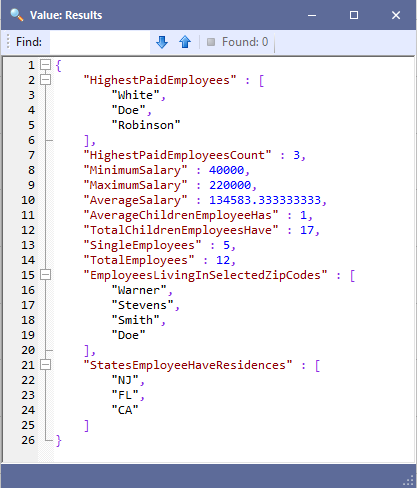
Output can be seen in the Parameter window, a parameter named “Results”.
Test Cases
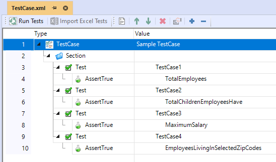
You can also run the defined test cases by navigating Test Case folder and open the TestCase.xml. Select the test case section and click on Run Tests. This TestCase file is setup against the Decision Graph approach. But you can change the logic file as required.
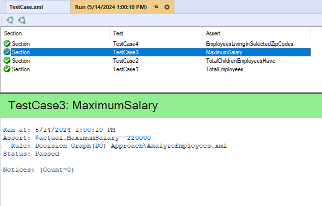
Then you can see the test results as follows.
Download
Use the attachment at the end of the page to download the sample project.